Project Overview :
● NumPy is an essential module for carrying out data science operations efficiently.
● NumPy stands for Numerical Python.
Matplotlib: Visualization with Python
● Matplotlib is a comprehensive library for creating static, animated, and interactive visualizations in Python. Matplotlib makes easy things easy and hard things possible. An object-oriented plotting library. A procedural interface is provided by the companion pyplot module, which may be imported directly. Eg: import matplotlib.pyplot as plt
Matplotlib Application Interfaces (APIs)
● Matplotlib has two major application interfaces, or styles of using the library:
● An explicit "Axes" interface that uses methods on a Figure or Axes object to create other Artists, and build a visualization step by step. This has also been called an "object-oriented" interface.
● An implicit "pyplot" interface that keeps track of the last Figure and Axes created, and adds Artists to the object it thinks the user wants.
Requirements :
● Python
● VS code
● Library – numpy and matplotlib
Code :
import numpy
import matplotlib.pyplot as plt

x = numpy.array([1,2,3,5,6,7,8,9,10,12,13,14,15,16,18,19,21,22])
y = numpy.array([100,90,80,60,60,55,60,65,70,70,75,76,78,79,90,99,99,100])

mymodel = numpy.poly1d(numpy.polyfit(x, y, 3))

myline = numpy.linspace(1, 20, 50)
print(myline)
plt.scatter(x, y)
plt.plot(myline, mymodel(myline))
plt.show()
Code Explanation :
● import numpy =>import numpy as np and use it in python. In command prompt or VS code terminal run the below pip command to install numpy library,
● pip3 install numpy # For Python version 3
● import matplotlib.pyplot as plt import matplotlib and use it in python. In command prompt or VS code terminal run the below pip command to install matplotlib library,
● pip3 install matplotlib
● Here pyplot() is the most important function in matplotlib library, which is used to plot 2D data.
● x = numpy.array([1,2,3,5,6,7,8,9,10,12,13,14,15,16,18,19,21,22]) -> Create the array that represent the values of the x
● y = numpy.array([100,90,80,60,60,55,60,65,70,70,75,76,78,79,90,99, 99,100]) -> Create the array that represent the values of the y axis.
Syntax : numpy.poly1d()
● class numpy.poly1d(c_or_r, r=False, variable=None)
● A one-dimensional polynomial class. A convenience class, used to encapsulate “natural” operations on polynomials so that said operations may take on their customary form in code (see Examples).
Parameters :
● c_or_r : The polynomial’s coefficients, in decreasing powers, or if the value of the second parameter is True, the polynomial’s roots (values where the polynomial evaluates to 0).
● r : bool, If True, c_or_r specifies the polynomial’s roots; the default is False.
● r : bool, If True, c_or_r specifies the polynomial’s roots; the default is False.
Syntax : numpy.polyfit()
● numpy.polyfit(x, y, deg, rcond=None, full=False, w=None, cov=False)
● The Polynomial.fit class method is recommended for new code as it is more stable numerically.
● x :array_like, shape (M,)
● x-coordinates of the M sample points (x[i], y[i]).
● y :array_like, shape (M,) or (M, K)
● y-coordinates of the sample points. Several data sets of sample points sharing the same x-coordinates can be fitted at once by passing in a 2D-array that contains one dataset per column.
● deg : int Degree of the fitting polynomial
● rcond : float
Relative condition number of the fit. Singular values smaller than this relative to the largest singular value will be ignored. The default value is len(x)*eps, where eps is the relative precision of the float type, about 2e-16 in most cases.
● full : bool
Switch determining nature of return value. When it is False (the default) just the coefficients are returned, when True diagnostic information from the singular value decomposition is also returned.
● w : array_like, shape (M,)
Weights. If not None, the weight w[i] applies to the unsquared residual y[i] - y_hat[i] at x[i]. Ideally the weights are chosen so that the errors of the products w[i]*y[i] all have the same variance. When using inverse-variance weighting, use w[i] = 1/sigma(y[i]). The default value is None.
● cov : bool or str, optional
If given and not False, return not just the estimate but also its covariance matrix. By default, the covariance are scaled by chi2/dof, where dof = M - (deg + 1), i.e., the weights are presumed to be unreliable except in a relative sense and everything is scaled such that the reduced chi2 is unity. This scaling is omitted if cov='unscaled', as is relevant for the case that the weights are w = 1/sigma, with sigma known to be a reliable estimate of the uncertainty.
● mymodel = numpy.poly1d(numpy.polyfit(x, y, 3))
Syntax : numpy.linspace()
● numpy.linspace(start, stop, num=50, endpoint=True, retstep=False, dtype=None, axis=0)
● Return evenly spaced numbers over a specified interval.
● Returns num evenly spaced samples, calculated over the interval [start, stop].
● The endpoint of the interval can optionally be excluded.
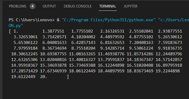
● myline = numpy.linspace(1, 20, 50)
● print(myline)
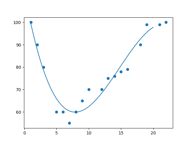
● plt.scatter(x, y)
● plt.plot(myline, mymodel(myline)) Plot the graph.
● plt.show()
● Run the code.
Output :
● After running the code, output of the terminal as given below,
● Graph was generated in the plot.